In our previous post we gave some details on the architectural decisions behind xcore.ai and its vector processing unit (VPU). The design aimed to deliver performance comparable to application processors, while keeping the price in the domain of small microcontrollers. While the price of the actual chip is critical, it is also essential keep in mind the costs of integration and customization, especially for a proprietary architecture like ours targeting vertical and platform solutions. Beyond the extensive IO libraries inherited from our previous generation of architectures and our port of FreeRTOS, xcore.ai comes with optimized math and DSP libraries, as well as neural network kernel libraries and easy-to-use machine learning model deployment tools. In this post, we will give more insight on the latter, both in terms of its implementation and how it’s used.
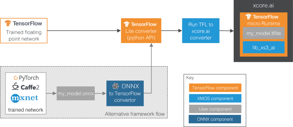
The figure below illustrates our neural network deployment workflow, starting with a trained model (with floating point weights and activations) on the left. Our workflow currently targets only TensorFlow models, so you need to convert your model first if you are training in a different framework. Once your model is in TensorFlow, the first step is to convert and quantize it using the built-in TFLite converter. You can do this manually, but we provide you with a helper function that takes a tf.keras Model object and a representative dataset for quantization, then configures and calls the converter/quantizer with the appropriate settings for xcore.ai.
Once your model is quantized, the next step is to use our converter to optimize the computational graph for our platform. The xcore.ai optimizer/converter consumes the model in the TFLite flatbuffer format output by the converter and outputs another flatbuffer following the same TFLite schema. The optimizer’s internal structure is similar to that of a compiler:
- The model is converted to our own intermediate representation (IR) of the computational graph
- Transformations are applied in multiple stages, each stage consisting of multiple passes that mutate the IR, including canonicalization, optimization, lowering, cleanup, and other passes.
- The IR is serialized (i.e. converted) back to the TFLite flatbuffer format.
The most important xcore.ai specific transformations performed are related to the optimization of convolutions and fully connected layers. Due to hardware ring buffer implementation of the VPU described in our previous post, the most efficient kernel implementation may require the weight tensor to be laid out differently from OHWI (i.e. output channel, kernel height, kernel width, input channel) layout used by TFLite. Moreover, some parameters related to quantization can be precalculated and stored interleaved with the biases, reducing overhead and speeding up execution. Beyond the transformation passes that calculate these custom weight, bias and quantization parameter tensors, our converter also plans the parallel execution of the kernels, fuses zero-padding operators with convolutions, and performs many other optimizations.
It is worth noting that our optimizer is a standalone executable with the input and output model in the same format. This means that you can use it even if you have custom operators in your model, e.g. the way binarized operators are represented in models trained with Larq. Our optimizer was designed to not alter unknown custom operators by default but be extensible if implementing optimizations for such operators is desired.
The final step in our conversion workflow is to deploy your model in our port of the TFLite for Microcontrollers (TFLM) runtime. The TFLM project provides the tools necessary to encapsulate the model and the runtime in source files that can be linked with the rest of your embedded project, compiled using our tools, and deployed on the hardware or tested in our cycle-accurate simulator. To execute the optimized graph, our TFLM runtime relies on a library of fine-tuned neural network kernels that take full advantage of the xcore.ai VPU. This library is also self-contained, so you can implement the model execution yourself if the computation constraints do not allow the overhead associated with the runtime. This overhead can be anything between 20KB and 160KB, depending on how many and which kernels your model uses, but decreases continuously as we improve our implementation of the runtime and the kernels.
For a step-by-step guide through the xcore.ai conversion workflow, check-out the recording of our TinyML Talks webcast here.