Same Input, Different Action – the role of timing determinism in physical AI

Run a trained neural network twice on the same input, with the same weights and the same random seed, and you get the same answer. Run a robot twice in the same situation and you may not. Some of that variation is deliberate, because many modern policies sample on purpose. Some of it comes from an input nobody declared: timing.

Earlier pieces in this series argued that physical AI needs a predictable reflex layer beneath its probabilistic reasoning, and that timing guarantees cannot be added after the fact to hardware never built to provide them. This piece makes a narrower, more mechanical case: timing is an undeclared input. When it varies, the same situation can produce a different action — and the standard workaround for unpredictable timing costs the one thing a fast control loop cannot spare: latency.  The trade runs one way only: you can always add a buffer; you cannot remove unpredictable timing without one.

Time is an input

Strip away the machine-learning vocabulary and the point is simple: time is an input, whether or not anyone declared it. Every model that consumes a stream of measurements assumes something about the spacing between them. A policy trained on periodic observations taken 200 times a second has learned what five thousandths of a second of the world looks like, and nothing else.

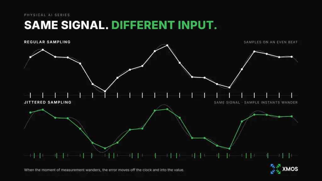
When the moment of measurement wanders, what engineers call jitter, the error does not stay on the clock. It becomes an error in the measured value, and the faster the signal is changing, the bigger the error. A drifting temperature tolerates sloppy timing; a contact transient, a surge of motor current or an acoustic wavefront does not.  For a 1 kHz vibration read by a software-timed sensor, sampling instants that wander by a millionth of a second (RMS) cap signal-to-noise at about 44 dB — the quality of a 7-bit converter, however many bits the converter actually has.

The distinction that matters most is between delay and variation in delay. A fixed delay — latency — can be measured once, compensated for in the controller and folded into the training data. A variable delay — jitter — is noise, and noise on the time axis cannot be calibrated away. That is why determinism is not the same as speed. A system that always responds in 500 microseconds is often more useful than one that averages 100 but occasionally takes 2,000. The first is a design parameter. The second is a failure mode with a probability that must be accommodated.

The obvious fix: stamp it, buffer it, line it up

The industry’s standard answer to unpredictable timing is rational and widely deployed. Stamp every measurement with its capture time; let it travel through whatever media, drivers and queues it must; hold it in a buffer; and once every sensor has delivered its slice of time, line the streams up on a common clock before handing them to the model. Most imaging pipelines do some version of this.

It works, up to a point. It restores the alignment of the data, but at a cost.

First, it removes jitter by converting it into delay. The buffer cannot release a slice until its latest measurement arrives. Size it for the typical case and late data is dropped or misaligned; size it for the worst case and every slice pays the worst-case latency, every time.

Second, it is only as good as the timestamp. A timestamp written by software after the processor has got round to noticing a measurement inherits exactly the delay it was meant to correct. It says nothing about when a given measurement was actually captured at the input, or when the code that processes it actually runs. Unless the stamp is applied in hardware at the moment of capture, the alignment step is addressing one wandering quantity with another.

Third, it fixes the input, not the output. Once the model has chosen an action, the command still travels back through drivers, queues and buses to the actuator, and that path wanders too. Aligning the inputs perfectly does not make the action land at a known instant. Making it do so means buffering again on the way out, and paying more latency.

The industry is not standing still. PTP gives devices a shared clock. EtherCAT’s distributed clocks latch drive inputs and outputs against it with sub-microsecond precision. Hardware triggers fire cameras and sensors together. Some teams feed the measured sample interval to the model as an extra input. These are real solutions, and where they apply they do make capture deterministic. What none of them does is make the whole path deterministic (the capture, the computation on it and the action that follows) across many different sensor streams at once. Timing is pinned down at the edges and left to chance in the middle. That is the gap.

Where delay is cheap, this is a perfectly good trade. The question is where it is not.

When waiting is not an option

In a one-way pipeline — transcribe this recording, label this image — delay is an inconvenience. In a feedback loop, where every action changes what the sensors see next, delay is a stability problem. Anyone who has tried to steer while watching the road on a lagging video feed knows the result: you correct, the correction arrives late, you over-correct, and you start to weave.

Control engineers can put numbers on it. Delay pushes a correction out of step with the disturbance it is meant to cancel, and the faster a loop has to respond, the more each millisecond costs. In a loop that must counter disturbances oscillating up to 100 times a second, one millisecond of delay shifts its correction by 36 degrees — more than a tenth of a cycle. Well-designed loops typically carry 45 to 60 degrees of safety margin, so a single millisecond can consume most of it, and less than two milliseconds can be enough to tip the loop into oscillation.

THE LATENCY LADDER

How long can the loop afford to wait?

MICROSECONDS	UNDER A MILLISECOND	MILLISECONDS	TENTHS OF A SECOND · BATCHING WORKS
Motor control and noise cancellation	Touch, force and balance	Grip and fast AI policies	Planning and reasoning
Current loops at tens of kHz; anti-noise that must beat the sound wave.	Haptics, force control and flight stabilisation.	Tightening grip when an object slides (slip reflex); vision-in, motor-out (visuomotor) policies at 100–200 Hz.	Scene understanding and task planning.

_{Indicative orders of magnitude. Batching is affordable only at the right-hand end — further left, the buffer alone can consume all the delay the loop can tolerate.}

The obvious counter-example: the most advanced humanoids already run their AI on GPUs and make movement decisions around 200 times a second, and they work. But underneath sit dedicated motor controllers correcting the joints thousands of times a second with predictable timing, quietly smoothing over the GPU’s irregularities. The predictable layer is already there; the question is how much it will have to carry as AI takes on faster, more delicate work like gripping and balancing. Faster chips will not close the gap – speed improves the typical response, but it is the occasional slow one that breaks a control loop.

Why small timing errors do not stay small

The intuitive defence of jitter is statistical: timing errors are tiny and random, so they average out. In a system that makes one-off judgements, that is roughly true. In a physical AI system it fails, because the errors pass through three mechanisms that amplify them, accumulate them and/or feed them back.

Rates amplify them. Controllers and AI policies care about how fast things are changing — velocity, acceleration, the rate at which force is building — and those rates are worked out by comparing successive measurements over an assumed constant interval. Suppose a stream sampled a thousand times a second assumes each step is exactly one millisecond, but each sample can land up to a tenth of a millisecond early or late. If one sample is early and the next is late, the gap between them is out by two tenths — so a velocity estimate can carry up to 20% error from timing alone, or 10% if only one sample of the pair is displaced.

Memory accumulates them. Many models, and the estimators that feed them, carry an internal state from one step to the next. An error injected there is remembered, and in quantities built up from small increments — position from velocity, orientation from rotation rate — it can accumulate. It is the same reason navigation from motion sensors alone steadily drifts.

The loop feeds them back. A robot’s action decides what it sees next. A timing error produces a slightly wrong action, then a slightly unfamiliar situation in which the model is less reliable, then a more wrong action. This drift away from training conditions is one of the best-documented weaknesses of learned control: since Ross and Bagnell’s 2010 analysis, it has been known that errors in imitation-trained policies can grow with the square of the task’s length.  Jitter is a plausible and largely unexamined source of that drift, and one the training data almost never contained.

A fair objection: train the model on deliberately jittered data and it learns to cope. It does, randomising timing and other conditions in training has been standard practice since Tan et al.’s 2018 work on legged robots. But robustness has a price, and Tan’s team saw it: randomisation made their robots more stable but less capable. A model tolerates noisy timing by paying less attention to its fastest, most timing-sensitive signals — in effect, blurring its own perception. It trades responsiveness for input tolerance. In tasks involving contact, responsiveness is the whole point.

One stream or many?

“Timing determinism” bundles two different properties; the first is regularity within a single stream: each sensor sampled on an even beat.  The second is coherence across streams: every sensor sharing one clock, sampled in a known, fixed relationship to every other.

Regularity within a stream matters most where one fast signal is processed largely on its own. A motor’s current loop filters and differentiates its measurements on the assumption of a fixed interval between them; vibration analysis for predictive maintenance converts a sensor’s signal into a frequency spectrum, which smears when the interval wanders. In both cases jitter corrupts the result before any other sensor is involved.

Cross-stream coherence dominates wherever meaning comes from comparing or combining signals. A microphone array locates a speaker from tiny differences in arrival time; at a typical audio sampling rate, one sample of misalignment is about seven millimetres of sound travel — a large fraction of what the array is measuring. Camera and motion-sensor fusion degrades when the two disagree about time by a few milliseconds. A dexterous hand detects slip by correlating fingertip shear with joint motion. Whole-body balance needs every joint controller to agree on when “now” is.

For physical AI, coherence across streams is the more important property and the harder one, for two reasons.

It cannot be fixed locally. A single wobbly stream can be re-timed onto an even beat where it was captured, given a hardware timestamp. Disagreement between streams needs a shared notion of time across physically separate devices — a property of the whole architecture, not of any one component.

Misaligned streams can corrupt model structure, not just weights. A model that combines senses learns the relationships between them: this sound came from there; this force followed that movement. Misalignment shifts those relationships in time and can even put an effect before its cause. A fixed offset is learnable, but a varying one teaches the model that the relationship is unreliable, so it learns to discount it – detracting from the very benefit that justified the extra sensors.

The exception is the innermost loop. In motor control and noise cancellation the loop is local and very fast, and single-stream regularity is what determines effectiveness. A useful rule of thumb: regularity governs the reflex; coherence governs perception. And as the previous piece in this series argued using the humanoid hand, every added touch sensor, joint and microphone is another stream that must agree on time with the rest – so coherence matters more with every sensor a robot gains.

The hardware has to keep time

If timing determines what the model sees, it has to be designed in where measurements are made, not reconstructed downstream. That means taking time at the pin – stamping measurements and scheduling actions in hardware, not in software after the fact; making any latency a constant the controller can absorb rather than a distribution it cannot; closing reflexes locally, never behind a buffer waiting for the slowest sensor; and designing-in coherence across streams from the outset, because it cannot be recovered one component at a time.

XCORE® is XMOS’s family of GenSoC™ processor platforms, in which every core and every I/O pin is timed by hardware rather than by an operating-system scheduler. In a robot it sits between the sensors and the GPU, at a hand, a joint cluster or a sensor array. There it captures many streams coherently, closes the reflexes locally and passes a clean, timestamped stream up to the reasoning layer. It does this in three specific ways.

Coherence across many streams. An XCORE device can be configured to capture many sensor streams at once — microphone arrays, touch sensors, motor encoders — through its own input ports, with each sample latched in hardware against a single on-chip reference. Coherence is built in at capture, not reconstructed afterwards, on a timer that is typically configured for 10ns resolution.  A value or values captured on XCORE IO can create a corresponding output event in as little as 20ns – a property that remains constant regardless of activity elsewhere in the device.

Across devices, for example one XCORE per hand or limb, the same timers can be disciplined to a shared reference through XMOS link technology. Coherence that is exact inside a device is then bounded and known between devices.

Reflex-layer inference on the same clock. The same device runs the small neural networks of the reflex layer — detecting a slip, a fault, an anomaly in a vibration signature — against that same clock, alongside control and signal processing. The time from measurement to action is a number known at design time, not a distribution discovered in the field.

Scheduled actions, and a clean split between fast and slow. XCORE’s output ports apply a command at a specified clock tick rather than whenever it happens to be ready. That lets the system be split honestly. The reflexes (slip, contact, current, balance) close locally, pin to pin, with no buffer and no wait for the slowest sensor. Commands from a GPU-based policy are released at a fixed offset from the timestamped measurement that produced them. That offset must cover the GPU’s worst case, so the slow path does pay in latency. But it pays a constant, known delay the controller can absorb, and nothing that keeps the robot stable is waiting behind it. Buffer where delay is cheap; never where it isn’t.

This is the asymmetry the piece began with. A predictable front end can always feed a buffered, timestamped stream to a reasoning layer that wants one. An unpredictable front end can only be cleaned up by incurring delay. You can always add a buffer; you cannot remove jitter without one.

Why not use the real-time cores already on a GPU module, or pair a microcontroller with an FPGA? Both can latch a timestamp at a pin, but neither puts a configurable set of sensor streams, control loops and small neural networks on one software-defined fabric sharing one clock, without splitting the work across chips and toolchains – wasting accuracy, energy and time to market.

What this actually means

The industry is rigorous about measuring its models and far less rigorous about the time axis they consume. Three numbers deserve the same scrutiny as accuracy, in the lab and in the field:

• Capture jitter: how far each sensor’s actual sample instants stray from its nominal beat.
• Cross-stream skew: how far apart two “simultaneous” samples from different sensors really are, and how much that varies.
• Measurement-to-action spread: the distribution, not the average, of time from a sample at the input pin to the resulting command at the output pin. Report the 99.9th percentile, not the mean.

Each can be measured with a GPIO toggle and a logic analyser. The same applies to the data a model learns from, because a demonstration recorded on a jittery stack bakes that jitter into the training set. We expect teams that measure these numbers to find that some of what they call brittle models is in fact timing.

Plenty of today’s robots work well on unpredictable computing stacks, but they rely on fast, deterministic motor drives to quietly absorb the damage, one joint at a time. That holds while the AI sits a layer or two above the reflex. It holds less well as policies get faster, closer to contact and more reliant on combining senses, which is exactly where physical AI is heading. A hand that feels slip across twenty fingertip sensors needs a reflex that no single joint’s drive can see. That is the layer XCORE is built for.

The model is not the whole system. Same situation, same action requires two kinds of determinism: functional — the model computes the same answer from the same input — and timing — each measurement captured, aligned, processed and acted on at a known instant. The industry has invested heavily in the first.  The second is the one it rarely measures.